1. Digital Elevation Models and Raster Imagery
* Main input data source being DEM (Digital Elevation Models) derived from Satellite and LIDAR sources.
* DEM’s measure the highest point below a nominal observer hovering the earth (data can include buildings and trees).
* Imported into software in square tile or irregular format.
* Variable resolution from 5m to 1km.
2. Mapping and Coordinate Systems
* GIS requirements for use on Australian terrain data.
* Incorporating Australian AGD66, AGD84 and GDA94 datums (GRS80 ellipsoid) and equivalent UTM projections for grid coordinates AMG66, AMG84 and MGA94.
* Operations to perform conversions between Grid coordinates (Eastings/Northings) and Geographical (Latitude/Longitude) using Redfearn’s formulae.
* Distance and Height Scale factors for accurate distance calculations on the ellipsoid.
3. Empirical Propagation Models
* ITU recommended Empirical Pathloss models such as Okumura-Hata and Longely-Rice
* Okumura-Hata
model variations for
# 150MHz < f < 1500MHz
# 30m < Htx <200m
# 1m < Hrx <10m
# 1km < d <20km
* COST 231 Hata model
for 1500MHz-2000MHz.
4. Knife Edge Diffraction
* Semi Deterministic pathloss models employ knife edge diffraction for evaluating hilly terrain and finding losses in shadowed regions.
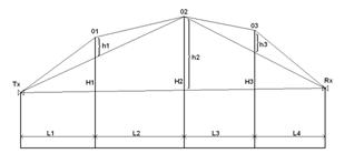
* A terrain cross section profile is produced between the Tx and Rx which is then passed through a convex hull function to find diffracting radio path.
* Decision calculations based on the knife edge model are performed to produce the Fresnel-Kirchoff diffraction parameter ν.
* Fresnel-Kirchoff parameter then substituted into Lee’s approximation of attenuation over single diffracting edge.
* Used in conjunction with the Friis transmission equation for pathloss (dependent upon Fresnel zone clearance).
Path loss (dB) = 32.44 + 20 log d (km) + 20 log f (MHz)
* Each model differs in its approach to determining the inputs to the Fresnel-Kirchoff diffraction parameter ν equation, and for what edge contributes most to the loss.
# Bullington model below takes simplest, least accurate approach and reduces the profile to a single knife edge
# Epstein-Peterson model below considers each significant knife edge individually and sums each loss over the diffracting path
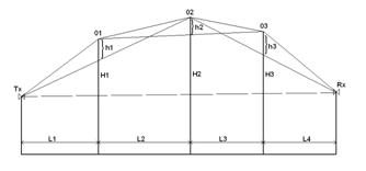
# Giovanelli method below identifies a dominant edge and calculates each loss wrt it, but creates seperate observation planes for each edge
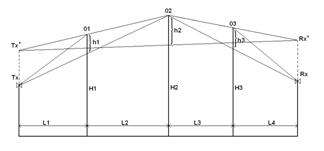
Deygout model below identifies a dominant knife edge and calculates all losses with respect to it.
5. Antenna modeling
* Vertical and Horizontal gain patterns loaded in from a manufacturers antenna data file.
* Pattern multiplication performed for a approximate 3D representation.
* Full gain pattern can be incorporated into propagation model via a simple raytrace function and added to the pathloss equation.